
File:Segment anisotropy.png
Original file (1,200 × 1,200 pixels, file size: 217 KB, MIME type: image/png)
Summary
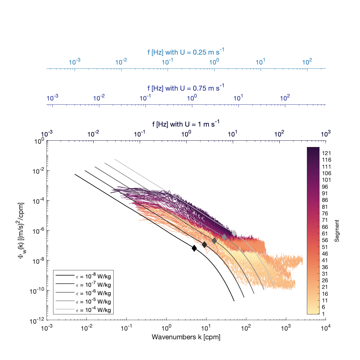
Example spectra for the Tidal shelf high-quality dataset. About 3h worth is shown, and each spectrum was constructed from 128 s (2.13min) worth of data, which was split into FFT-length of 32 s (2048 samples). The speeds past the sensor vary from a minimum of 0.3 m/s and a maximum of 0.8 m/s. The combination of high [math]\displaystyle{ \varepsilon }[/math] and fast speeds enables using short segments to compute the spectra. The impact of turbulence anisotropy is also visible with the flattening of the spectra at wavenumbers around 1 cpm.
File history
Click on a date/time to view the file as it appeared at that time.
| Date/Time | Thumbnail | Dimensions | User | Comment | |
|---|---|---|---|---|---|
| current | 16:35, 5 July 2022 | | 1,200 × 1,200 (217 KB) | CynthiaBluteau (talk | contribs) | Example spectra for the Tidal shelf high-quality dataset. About 3h worth is shown, and each spectrum was constructed from 128 s (2.13min) worth of data, which was split into FFT-length of 32 s (2048 samples). The speeds past the sensor vary from a minimum of 0.3 m/s and a maximum of 0.8 m/s. The combination of high <math>\varepsilon<\math> and fast speeds enables using short segments to compute the spectra. |
You cannot overwrite this file.
File usage
The following page uses this file: