File list
From Atomix
This special page shows all uploaded files.
| Date | Name | Thumbnail | Size | User | Description | Versions |
|---|---|---|---|---|---|---|
| 17:40, 9 June 2024 | Rolf Lueck.jpeg (file) |  |
131 KB | Rolf (talk | contribs) | Picture of Rolf Lueck | 1 |
| 21:00, 29 September 2023 | Flowchart symbol.png (file) |  |
36 KB | KikiSchulz (talk | contribs) | Symbolic representation of a data processing flowchart | 1 |
| 09:19, 29 September 2023 | ATOMIX load.txt (file) | 10 KB | Ilker (talk | contribs) | A Matlab function to load a grouped NetCDF file prepared following the recommendations of the shear probe group. It can be used to load a benchmark data file. Remember to change the extension to "m". | 1 | |
| 20:18, 9 December 2022 | Figure 381.jpg (file) |  |
1.51 MB | Rolf (talk | contribs) | The ratio of the true dissipation rate to the rate determined by integrating the spectrum to only 10 cpm, as a function of the 10-cpm rate for a range of kinematic viscosities. if the measured spectrum follows the Nasmyth spectrum. | 1 |
| 20:07, 9 December 2022 | Epsilon 10 to epsilon ratio.pdf (file) | 130 KB | Rolf (talk | contribs) | The ratio of the true dissipation rate to the dissipation rate determined by only integrating the spectrum of shear to 10 cpm, as a function of the 10cpm-rate for a range of kinematic viscosities. | 1 | |
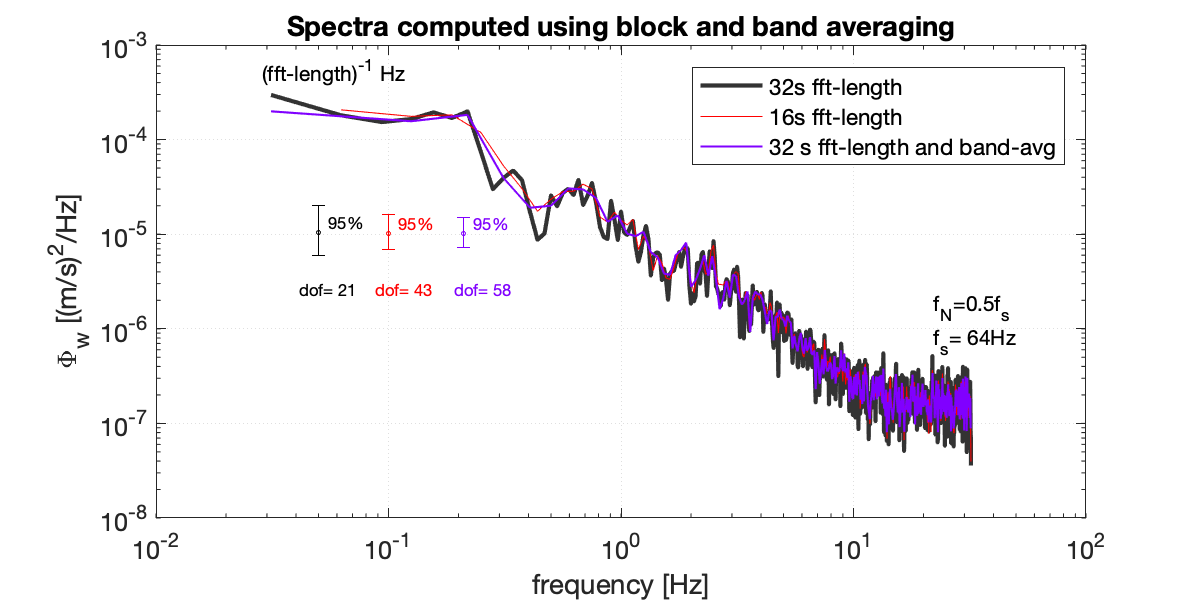
| 14:31, 11 July 2022 | Spectra computation.png (file) |  |
78 KB | CynthiaBluteau (talk | contribs) | Added labels for the fft-length, degrees of freedom and nyquist frequency <math>f_N</math> | 2 |
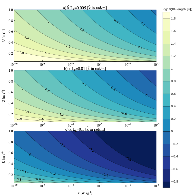
| 20:59, 10 July 2022 | ADV fft length.png (file) |  |
166 KB | CynthiaBluteau (talk | contribs) | Contours represent the log of the fft-length required to resolve the non-dimensional wavenumber [rad/m] indicated in each panel's title. The contours are plotted as a function of <math>\varepsilon</math> and speed past the sensor u. The fft-length controls the lowest frequency that is resolved by the spectra. The bottom panel (c) shows the fft-length that begins to resolve the viscous subrange i.e., the end of the inertial subrange. The middle panel shows the fft-length to resolve 1 decade'... | 1 |
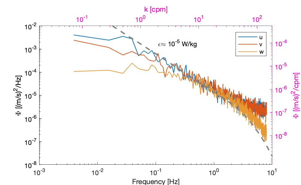
| 18:21, 5 July 2022 | Anisotropy.png (file) |  |
59 KB | CynthiaBluteau (talk | contribs) | Example of how turbulence anisotropy influenced the spectral shapes. This instrument was located very close to the bed (0.15 m) in a shallow waterway less than 2 m deep, which results in the vertical velocity's inertial subrange being reduced by the flattening of the spectra at wavenumbers of 10 cpm (0.1m scales). Strong stratification is another mechanism that shortens the inertial subrange at the lower wavenumbers. The wavenumber at which i... | 1 |
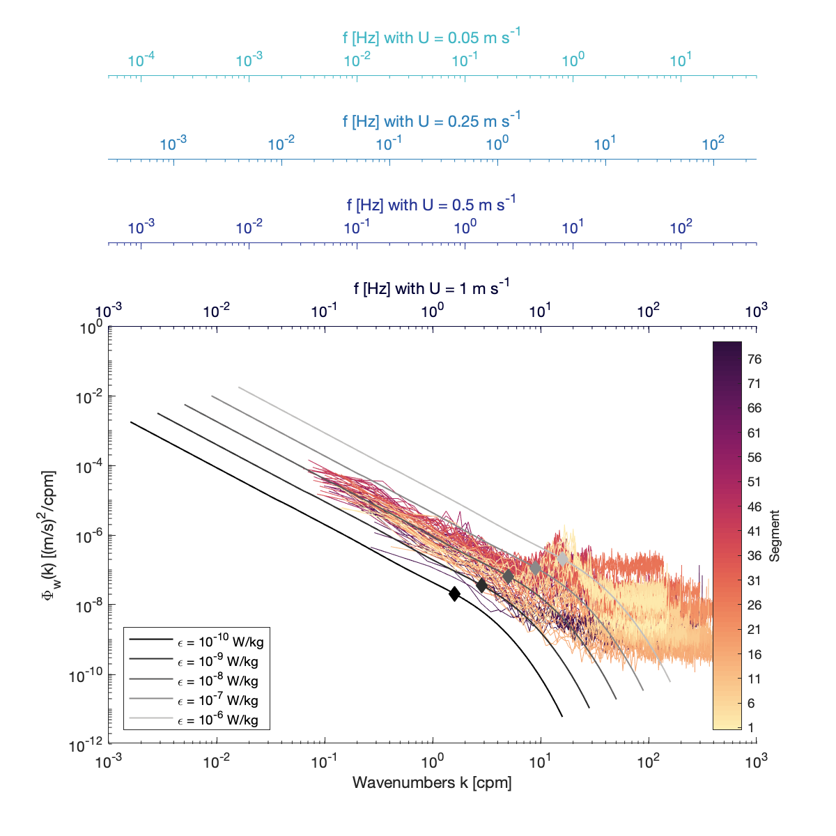
| 17:41, 5 July 2022 | SegmentAnisotropyLowE.png (file) |  |
207 KB | CynthiaBluteau (talk | contribs) | Example spectra for the Under-ice MAVS dataset. About 17h worth of segments are shown, and each spectrum was constructed from 1024 s (17.06 min) worth of data, which was split into FFT-length of 512s (4096 samples). The speeds past the sensor are of the order of a few cm/s. The combination of low <math>\varepsilon</math> and low speeds requires using relatively long segments to compute the spectra. The spectra are also impacted by vibrations and vortex shedding that are contaminating the meas... | 1 |
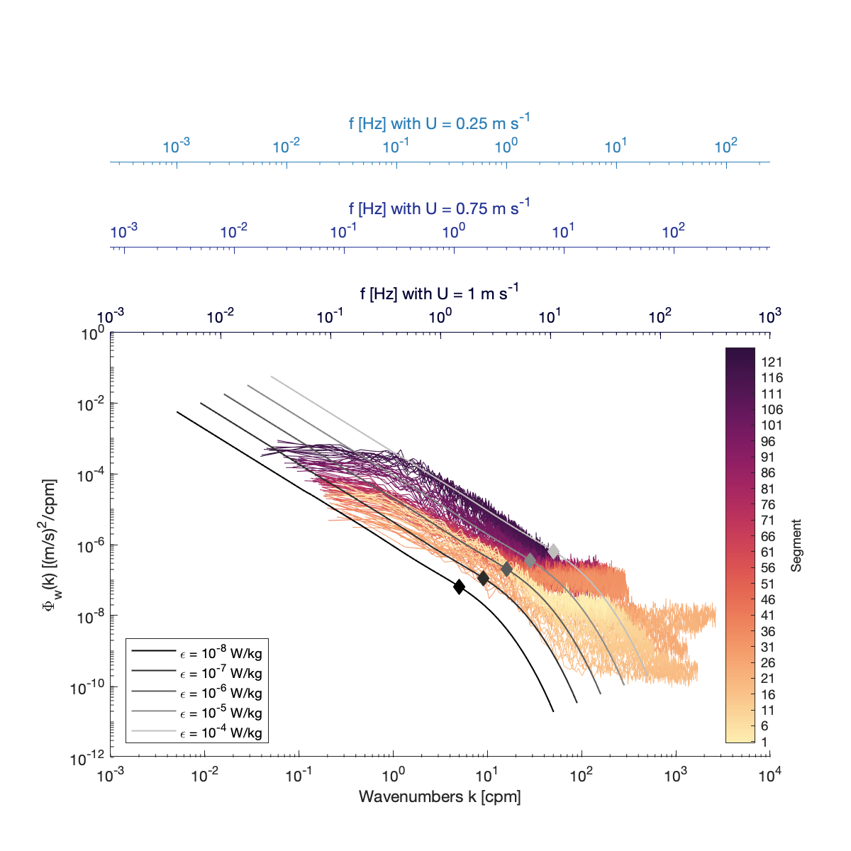
| 16:35, 5 July 2022 | Segment anisotropy.png (file) |  |
217 KB | CynthiaBluteau (talk | contribs) | Example spectra for the Tidal shelf high-quality dataset. About 3h worth is shown, and each spectrum was constructed from 128 s (2.13min) worth of data, which was split into FFT-length of 32 s (2048 samples). The speeds past the sensor vary from a minimum of 0.3 m/s and a maximum of 0.8 m/s. The combination of high <math>\varepsilon<\math> and fast speeds enables using short segments to compute the spectra. | 1 |
| 15:22, 5 July 2022 | Spectra replacement strategies.png (file) |  |
275 KB | CynthiaBluteau (talk | contribs) | Added panel labels | 2 |
| 14:59, 5 July 2022 | Timeseries replacement strategies.png (file) |  |
119 KB | CynthiaBluteau (talk | contribs) | Example velocity time series where we randomly removed data in varying length gaps. Only the example of 1min (480 samples at 8Hz sampling) are illustrated. Removing chunks of 8 continuous samples (1s) looks identical to the original time series and is not illustrated. | 1 |
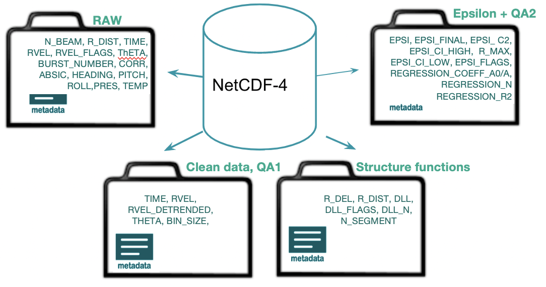
| 13:56, 23 May 2022 | ADCP netcdf variables.png (file) |  |
464 KB | Yuengdjern (talk | contribs) | 1 | |
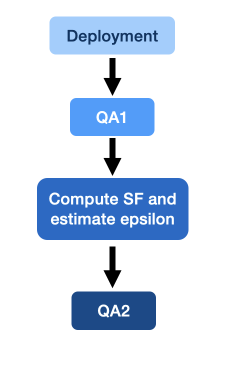
| 09:16, 23 May 2022 | ADCP SF flow chart.png (file) |  |
39 KB | Yuengdjern (talk | contribs) | 1 | |
| 08:55, 23 May 2022 | ADCP netcdf.png (file) |  |
502 KB | Yuengdjern (talk | contribs) | 1 | |
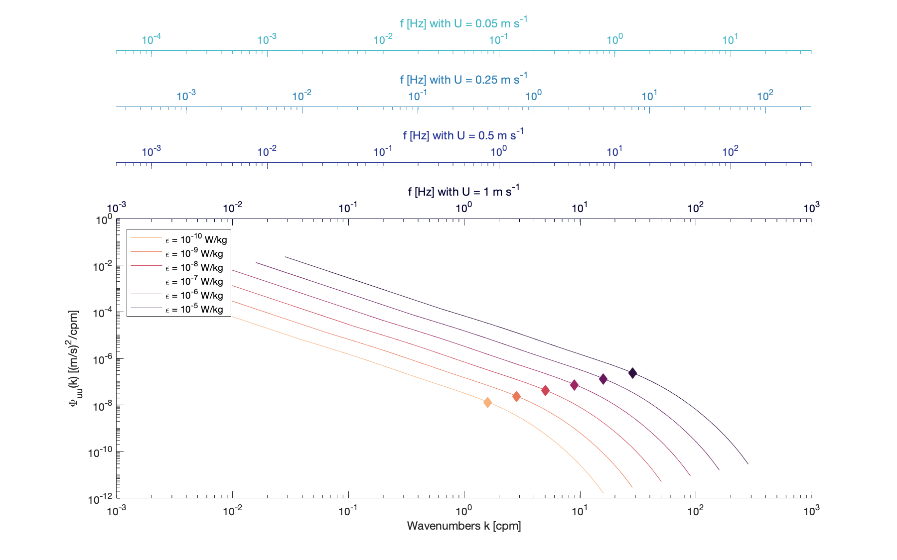
| 14:45, 23 March 2022 | IDM dimensional.png (file) |  |
92 KB | CynthiaBluteau (talk | contribs) | Added a smaller velocity of 0.05m/s for the secondary x-axes | 5 |
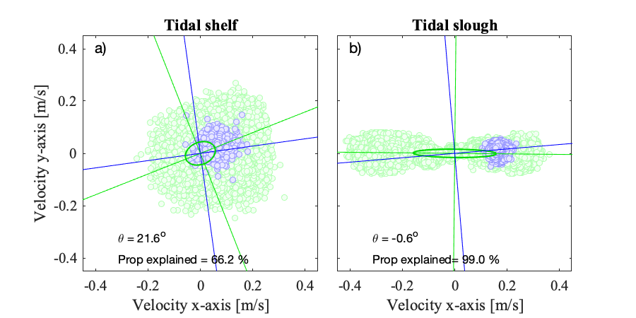
| 15:21, 8 March 2022 | Frame of reference adv.png (file) |  |
71 KB | CynthiaBluteau (talk | contribs) | Changed colors after some comments.. | 3 |
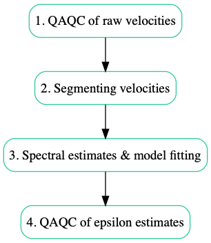
| 16:13, 5 March 2022 | Advprocessing.png (file) |  |
24 KB | CynthiaBluteau (talk | contribs) | Flowchart sketch for the landing page | 1 |
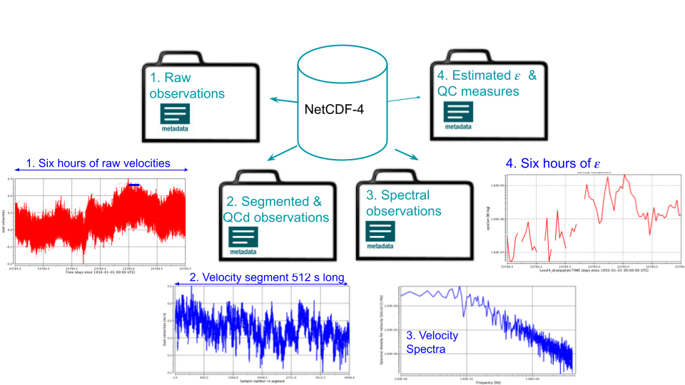
| 00:57, 3 March 2022 | Benchmark adv netcdf.png (file) |  |
131 KB | CynthiaBluteau (talk | contribs) | sketch of NetCDF format for point-velocity measurements | 1 |
| 22:18, 14 February 2022 | SF Fit JMM.png (file) |  |
61 KB | Jmmcmillan (talk | contribs) | 1 | |
| 17:24, 30 December 2021 | Kirstin.jpg (file) |  |
2.58 MB | KikiSchulz (talk | contribs) | Kiki profile pic | 1 |
| 20:12, 17 December 2021 | CBluteau.jpg (file) |  |
234 KB | CynthiaBluteau (talk | contribs) | Profile picture. | 1 |
| 14:26, 10 December 2021 | Yueng.jpg (file) |  |
6.52 MB | Yuengdjern (talk | contribs) | 2 | |
| 16:02, 7 December 2021 | Velocity spectra fft segment.png (file) |  |
91 KB | CynthiaBluteau (talk | contribs) | Accompanies File:Velocitie_fft_segment.png to illustrate the impact of increased FFT in the "smoothness" of the spectra and loss of spectral information at the lowest frequencies. Error bars also reduce with the increasing number of FFTs. The green... | 1 |
| 15:58, 7 December 2021 | Velocitie fft segment.png (file) |  |
55 KB | CynthiaBluteau (talk | contribs) | Vertical velocity records (8192 samples at 8Hz) to illustrate the use of smaller subsets of to compute FFTs. 50% overlap and hanning window applied to each fft-segment of data. The 15 FFTs example (cold color tones) uses 1024 samples (128 s) of records... | 1 |
| 18:40, 1 December 2021 | Velocity timescales.png (file) |  |
66 KB | CynthiaBluteau (talk | contribs) | Example velocity observations from an instrument impacted by tides and surface waves, which are presented as variance preserving spectra. The goal is to highlight when turbulence subranges begin in the grand scheme of physical processes that impact vel... | 1 |
| 20:59, 29 November 2021 | Short spectra.png (file) |  |
49 KB | CynthiaBluteau (talk | contribs) | Spectra of the short_timeseries.png to highlight the impact of detrending the entire timeseries first before segmenting onto 8.53 min (2048 samples) | 1 |
| 20:56, 29 November 2021 | Short detrend timeseries.png (file) |  |
84 KB | CynthiaBluteau (talk | contribs) | The detrended version of File:short_timeseries.png | 1 |
| 20:55, 29 November 2021 | Short timeseries.png (file) |  |
68 KB | CynthiaBluteau (talk | contribs) | Same as long_timeseries but showing only the first 512 s of data at 4Hz. | 1 |
| 17:22, 29 November 2021 | Long timeseries.png (file) |  |
89 KB | CynthiaBluteau (talk | contribs) | Example of velocities subsampled at 4Hz. Original timeseries measured at 64Hz, but lower sampling rate would be sufficient for IDM analysis. The different lines represent the results of various detrending. | 1 |
| 00:31, 25 November 2021 | Threshold logic Brock1986.png (file) |  |
37 KB | CynthiaBluteau (talk | contribs) | Fixed the threshold so that the local minimum is used for identifying thresholds, as opposed to the local minimum that reaches zero (ideal!) | 2 |
| 21:17, 24 November 2021 | Smoothed velocities.png (file) |  |
109 KB | CynthiaBluteau (talk | contribs) | Fixed legends, and identified the spikes on the bottom panel. | 3 |
| 19:03, 24 November 2021 | Despike spectra.png (file) |  |
48 KB | CynthiaBluteau (talk | contribs) | Example velocity spectra before and after removing a modest number of spikes (30x over 4096 samples) | 1 |
| 18:34, 24 November 2021 | Velocities spike.png (file) |  |
52 KB | CynthiaBluteau (talk | contribs) | Increased font size and reduced size. | 2 |
| 18:48, 22 November 2021 | SF atomix ADCP.png (file) |  |
90 KB | CynthiaBluteau (talk | contribs) | 2 | |
| 11:17, 13 November 2021 | Forward diff.png (file) | 175 KB | Brian scannell (talk | contribs) | 4 | ||
| 17:13, 12 November 2021 | Velocity data.png (file) |  |
154 KB | Brian scannell (talk | contribs) | 4 | |
| 16:49, 12 November 2021 | InertialSubrangeSchematic.png (file) |  |
60 KB | Jmmcmillan (talk | contribs) | Schematic of the velocity spectra in the inertial subrange | 1 |
| 16:16, 12 November 2021 | InertialSubrange.png (file) |  |
60 KB | Jmmcmillan (talk | contribs) | Removed 'equilibrium range' and updated axes labels to match equations. | 2 |
| 02:03, 11 November 2021 | ADCPschematic SF.png (file) |  |
77 KB | Jmmcmillan (talk | contribs) | Definition of structure function variables for a diverging beam. | 1 |
| 16:27, 10 November 2021 | Arnaud Pic.jpg (file) |  |
647 KB | Aleboyer (talk | contribs) | 1 | |
| 00:30, 9 November 2021 | Stationarity Figs.png (file) |  |
334 KB | CraigStevens (talk | contribs) | 1 | |
| 04:10, 23 October 2021 | Epsilometer EpsiFish FastCTDWinch.jpg (file) |  |
238 KB | Aleboyer (talk | contribs) | 1 | |
| 04:08, 20 October 2021 | UpwardsVMP250(DoubtfulSound-CLS).JPG (file) | .JPG) |
6.25 MB | CraigStevens (talk | contribs) | Upwards profiling VMP250 & Rebecca McPherson in DoubtfulSound (CLS, 5 September 2015) | 1 |
| 03:58, 20 October 2021 | NortekRope(CLS).JPG (file) | .JPG) |
1.29 MB | CraigStevens (talk | contribs) | Nortek Vector mounted on a line. (Stevens, 31 October 2011). | 1 |
| 03:45, 20 October 2021 | VMP500-CookSt.JPG (file) |  |
61 KB | CraigStevens (talk | contribs) | VMP 500 being deployed in Cook Strait in rough weather. (Stevens) | 1 |
| 03:42, 20 October 2021 | VMP 2000.jpg (file) |  |
177 KB | CraigStevens (talk | contribs) | Rockland VMP 2000(?) - Rudi Jozef Maria Caeyers. | 1 |
| 03:39, 20 October 2021 | RSI 5 float.jpg (file) |  |
299 KB | CraigStevens (talk | contribs) | Rockland MicroRider on profiling float. c/- RSI. | 1 |
| 03:36, 20 October 2021 | MSS ADCP CTD (Schaffer).JPG (file) | .JPG) |
7 MB | CraigStevens (talk | contribs) | MSS_ADCP_CTD_in_OceanCity_CC-BY Janin_Schaffer | 1 |
| 03:33, 20 October 2021 | AdcpMTOrig.png (file) |  |
114 KB | CraigStevens (talk | contribs) | Nortek signature ADCP in bottom-mounted frame. | 1 |

