Stationarity

Short definition of Stationarity
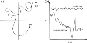
Stationarity refers to a constancy of statistical properties in any time (or space) series.

This is the common definition for Stationarity, but other definitions maybe discussed within the wiki.

Stationarity in the context of ocean turbulence refers to a constancy of statistical properties. The classic text on turbulence Tennekes and Lumley makes the point that "we would like to predict transport in real flows, which generally are inhomogeneous and nonstationary". It then goes on to focus on idealised, homogeneous, stationary situations. While many advances have been made in the subsequent 50 years, it is fair to say that this big-picture limitation remains.

(a) a particle moving in space and time (after Tennekes and Lumley, 1972) and (b) timeseries of velocity for stationary and non-stationary timeseries (after Kundu and Cohen 2004).

From the perspective of ocean turbulence the degree of stationarity needs to quantified in order to provide an indication of the viability of spectral approaches that assume stationarity. One way this quality control measure can be achieved is by varying the length of record section being examined and seeing if spectral properties vary substantially. Explicit examination of the issue in an oceanic context is not common. More attention is paid in atmospheric boundary layers where the lack of an inertial subrange, or the lack of a "spectral gap" between driving processes and turbulence are considered indicators. However, the scales of processes in the ocean precludes the use of a spectral gap. There have been efforts in assessing the impacts and benefits of filtering for stationarity in temperature microstructure sampling.

An example approach for velocimeters systematically accounting for departures from stationarity is described by Algot et al. (2017) These authors compare the 15 min time-evolution of one minute long statistics (mean and root-mean-square, r.m.s.) to those calculated identically from synthetic Gaussian noise time series. Because the Gaussian synthetic time series can differ for a given realization, they repeated the calculation 1000 times and used the average value. A threshold on the difference needs to be determined from known examples.

Another issue relating to stationarity is when the mean flow changes direction throughout the segment. Such segments can be excluded by invoking directional window over the data segment. Finally, flow disturbance by the mounting can induce rapidly varying spectral content.