Detrending time series: Difference between revisions
No edit summary |
|||
| (4 intermediate revisions by the same user not shown) | |||
| Line 5: | Line 5: | ||
}} | }} | ||
In the context of analysing turbulence observations, the resulting detrended signal should be [[stationary]] and contain mostly contributions from turbulence and surface waves (if present). However, frame interference (wakes), vibrations and measurement noise may also contaminate the detrended signal. | In the context of analysing turbulence observations, the resulting detrended signal should be [[Stationarity|stationary]] and contain mostly contributions from turbulence and surface waves (if present). However, frame interference (wakes), vibrations and measurement noise may also contaminate the detrended signal. | ||
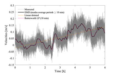
[[File:Long timeseries.png|thumb | [[File:Long timeseries.png|400px|thumb|Measured velocities at 4 Hz from an [[Acoustic-Doppler Velocimeters]] are highlighted against trends obtained from three different techniques. Empirical modal decomposition (EMD) <ref name="Wuetal_PNAS">{{Cite journal | ||
|authors=Zhaohua Wu, Norden E. Huang, Steven R. Long, and Chung-Kang Peng | |authors=Zhaohua Wu, Norden E. Huang, Steven R. Long, and Chung-Kang Peng | ||
|journal_or_publisher=PNAS | |journal_or_publisher=PNAS | ||
| Line 13: | Line 13: | ||
|year=2007 | |year=2007 | ||
|doi=10.1073/pnas.0701020104 | |doi=10.1073/pnas.0701020104 | ||
}}</ref>, linear trend, and a 2nd order low-pass Butterworth filter. A cut-off period of 10 min was targeted by both the filter and EMD]] | }}</ref>, linear trend, and a 2nd order low-pass Butterworth filter. A cut-off period of 10 min was targeted by both the filter and EMD. Detrended signal would be the difference between the original and the trend]] | ||
There is no exact definition for what consists of a "trend", nor any set algorithm for identifying the trend. The following techniques can be used for detrending <ref name=Wuetal_PNAS/>: | |||
# Linear trend removal | |||
# Low-pass linear filters | |||
# Empirical modal decomposition | |||
The first two methods presume the original time series is [[Stationarity|stationary]] and linear, while the third is adaptive and applicable to nonlinear and non-stationary time series. Note that chopping a time series into smaller subsets, i.e., segments, is essentially a form of low-pass (box-car) filtering. | |||
==Implications for estimating <math>\varepsilon</math>== | |||
===Velocity point measurements=== | |||
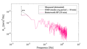
The choice of detrending technique has little influence on the estimation of <math>\varepsilon</math> from the spectral fitting of the inertial subrange as it influences only the lowest wavenumber of the spectra, which most algorithms identity as outliers. Detrending becomes an important consideration when performing other turbulence calculations such as estimating Re stresses <math>\overline{u'w'}</math> or turbulent kinetic energy. | |||
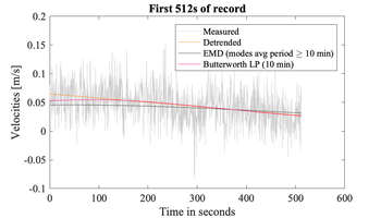
[[File:Short timeseries.png|left|thumb|350px|512 s segment of the measured velocities after applying different [[Detrending time series|detrending methods]]]] | |||
[[File:Short_spectra.png|left|thumb|350px|Example velocity spectra of the short 512 s of records before and after different <span id="detrend_ex">detrending</span> techniques applied to the original 6h time series. The impact of the detrending method can be seen at the lowest frequencies only]] | |||
===Velocity profilers=== | |||
==Notes== | ==Notes== | ||
Latest revision as of 14:39, 11 July 2022
| ({{{parameter_name}}})| }} |
|---|
| Detrending typically refers to removing the low-frequency content of the time series |
This is the common definition for Detrending time series, but other definitions maybe discussed within the wiki.
{{#default_form:DefineConcept}} {{#arraymap:Velocity point-measurements, Velocity profilers|,|x||}}
In the context of analysing turbulence observations, the resulting detrended signal should be stationary and contain mostly contributions from turbulence and surface waves (if present). However, frame interference (wakes), vibrations and measurement noise may also contaminate the detrended signal.

There is no exact definition for what consists of a "trend", nor any set algorithm for identifying the trend. The following techniques can be used for detrending <ref name=Wuetal_PNAS/>:
- Linear trend removal
- Low-pass linear filters
- Empirical modal decomposition
The first two methods presume the original time series is stationary and linear, while the third is adaptive and applicable to nonlinear and non-stationary time series. Note that chopping a time series into smaller subsets, i.e., segments, is essentially a form of low-pass (box-car) filtering.
Implications for estimating <math>\varepsilon</math>
Velocity point measurements
The choice of detrending technique has little influence on the estimation of <math>\varepsilon</math> from the spectral fitting of the inertial subrange as it influences only the lowest wavenumber of the spectra, which most algorithms identity as outliers. Detrending becomes an important consideration when performing other turbulence calculations such as estimating Re stresses <math>\overline{u'w'}</math> or turbulent kinetic energy.


