Decomposing velocity measurements: Difference between revisions
m Simplifying |
|||
| Line 4: | Line 4: | ||
}} | }} | ||
The quality-controlled velocities | The quality-controlled velocities can be [[Detrending time series|detrended]] before being further analysed to determine [[Velocity past the sensor|mean flow past the sensor]] and [[Surface wave statistics|surface wave statistics]]. These quantities are necessary for later choosing the appropriate [[Velocity inertial subrange model| inertial subrange model]] for [[Spectral fitting|spectral fitting]]. | ||
==Methods for detrending== | ==Methods for detrending== | ||
| Line 10: | Line 10: | ||
There is no exact definition for what consists of a "trend", nor any set algorithm for identifying the trend. The following techniques can be used for detrending <ref name=Wuetal_PNAS/>: | There is no exact definition for what consists of a "trend", nor any set algorithm for identifying the trend. The following techniques can be used for detrending <ref name=Wuetal_PNAS/>: | ||
# Linear trend removal | # Linear trend removal | ||
# Low-pass linear filters | # Low-pass linear filters | ||
# Empirical modal decomposition | # Empirical modal decomposition | ||
The first two methods presume the original time series is [[Stationarity|stationary]] and linear, while the third is adaptive and applicable to nonlinear and non-stationary timeseries. | The first two methods presume the original time series is [[Stationarity|stationary]] and linear, while the third is adaptive and applicable to nonlinear and non-stationary timeseries. | ||
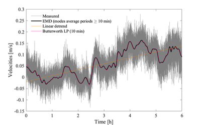
[[File:Long timeseries.png|400px|thumb|Measured velocities at 4 Hz from an [[Acoustic-Doppler Velocimeters]] have been detrended using three different techniques. Empirical modal decomposition (EMD) <ref name="Wuetal_PNAS">{{Cite journal | [[File:Long timeseries.png|400px|thumb|Measured velocities at 4 Hz from an [[Acoustic-Doppler Velocimeters]] have been detrended using three different techniques. Empirical modal decomposition (EMD) <ref name="Wuetal_PNAS">{{Cite journal | ||
| Line 23: | Line 23: | ||
}}</ref>, linear trend, and a 2nd order low-pass Butterworth filter. A cut-off period of 10 min was targeted by both the filter and EMD]] | }}</ref>, linear trend, and a 2nd order low-pass Butterworth filter. A cut-off period of 10 min was targeted by both the filter and EMD]] | ||
== | ==Application to measured velocities== | ||
Measurements are typically collected in the following two ways: | |||
* continuously, or in such long bursts that they can be considered continuous | |||
* short bursts that are typically at most 2-3x the expected largest turbulence time scales. | |||
As a rule of thumb, turbulence estimates from the inertial subrange of velocity rely on 5 to 15 min long-[[Segmenting datasets|segments]]. | |||
==Segmenting== | ==Segmenting== | ||
Revision as of 20:50, 29 November 2021
{{#default_form:Processing}}
{{#arraymap:
{{#switch: ADV | ADV=Velocity point-measurements |ADCP= Velocity profilers | Shear=Shear probes}}
|,|x||}}
{{#if: level 2 segmented and quality controlled | {{#arraymap:level 2 segmented and quality controlled|,|x||}}}}
The quality-controlled velocities can be detrended before being further analysed to determine mean flow past the sensor and surface wave statistics. These quantities are necessary for later choosing the appropriate inertial subrange model for spectral fitting.
Methods for detrending
There is no exact definition for what consists of a "trend", nor any set algorithm for identifying the trend. The following techniques can be used for detrending <ref name=Wuetal_PNAS/>:
- Linear trend removal
- Low-pass linear filters
- Empirical modal decomposition
The first two methods presume the original time series is stationary and linear, while the third is adaptive and applicable to nonlinear and non-stationary timeseries.

Application to measured velocities
Measurements are typically collected in the following two ways:
- continuously, or in such long bursts that they can be considered continuous
- short bursts that are typically at most 2-3x the expected largest turbulence time scales.
As a rule of thumb, turbulence estimates from the inertial subrange of velocity rely on 5 to 15 min long-segments.
Segmenting
Chopping timeseries into smaller segments is essentially a form of filtering (box-car).
Notes
<references/>
