File:Segment anisotropy.png: Difference between revisions
From Atomix
m →Summary |
m →Summary |
||
| Line 1: | Line 1: | ||
== Summary == | == Summary == | ||
Example spectra for the Tidal shelf high-quality dataset. About 3h worth is shown, and each spectrum was constructed from 128 s (2.13min) worth of data, which was split into FFT-length of 32 s (2048 samples). The speeds past the sensor vary from a minimum of 0.3 m/s and a maximum of 0.8 m/s. The combination of high <math>\varepsilon</math> and fast speeds enables using short segments to compute the spectra. The impact of [[#anisotropy|turbulence anisotropy]] is also visible with the flattening of the spectra at wavenumbers around 1 cpm. | Example spectra for the Tidal shelf high-quality dataset. About 3h worth is shown, and each spectrum was constructed from 128 s (2.13min) worth of data, which was split into FFT-length of 32 s (2048 samples). The speeds past the sensor vary from a minimum of 0.3 m/s and a maximum of 0.8 m/s. The combination of high <math>\varepsilon</math> and fast speeds enables using short segments to compute the spectra. The impact of [[Velocity inertial subrange model#anisotropy|turbulence anisotropy]] is also visible with the flattening of the spectra at wavenumbers around 1 cpm. | ||
Latest revision as of 17:27, 5 July 2022
Summary
Example spectra for the Tidal shelf high-quality dataset. About 3h worth is shown, and each spectrum was constructed from 128 s (2.13min) worth of data, which was split into FFT-length of 32 s (2048 samples). The speeds past the sensor vary from a minimum of 0.3 m/s and a maximum of 0.8 m/s. The combination of high and fast speeds enables using short segments to compute the spectra. The impact of turbulence anisotropy is also visible with the flattening of the spectra at wavenumbers around 1 cpm.
File history
Click on a date/time to view the file as it appeared at that time.
| Date/Time | Thumbnail | Dimensions | User | Comment | |
|---|---|---|---|---|---|
| current | 16:35, 5 July 2022 | 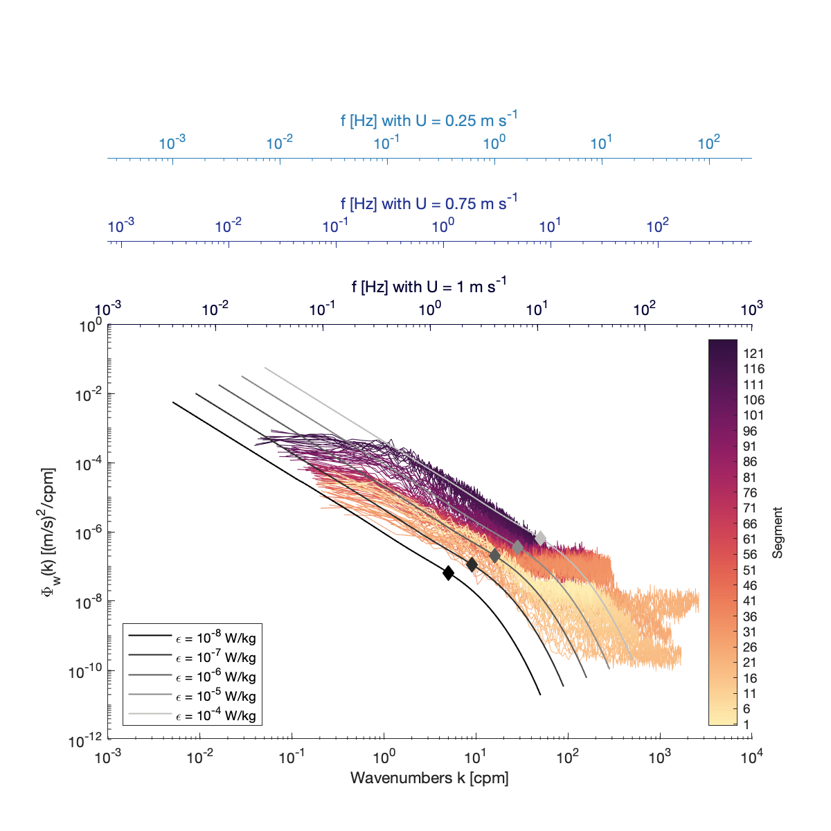 | 1,200 × 1,200 (217 KB) | CynthiaBluteau (talk | contribs) | Example spectra for the Tidal shelf high-quality dataset. About 3h worth is shown, and each spectrum was constructed from 128 s (2.13min) worth of data, which was split into FFT-length of 32 s (2048 samples). The speeds past the sensor vary from a minimum of 0.3 m/s and a maximum of 0.8 m/s. The combination of high <math>\varepsilon<\math> and fast speeds enables using short segments to compute the spectra. |
You cannot overwrite this file.
File usage
The following page uses this file:

