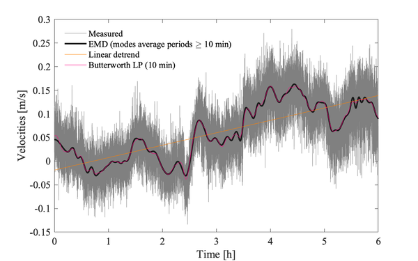
Decomposing velocity measurements: Difference between revisions
| Line 19: | Line 19: | ||
|doi=10.1073/pnas.0701020104 | |doi=10.1073/pnas.0701020104 | ||
}}</ref>, linear trend, and a 2nd order low-pass Butterworth filter. A cut-off period of 10 min was targeted by both the filter and EMD]] | }}</ref>, linear trend, and a 2nd order low-pass Butterworth filter. A cut-off period of 10 min was targeted by both the filter and EMD]] | ||
===Long continuous sampling=== | ===Long continuous sampling=== | ||
'''Info needs simplifying after convening as a subgroup''' | |||
Different techniques dependent on whether measurements were collected continuously or in long bursts (define here). The high-frequency content can be obtained by: | Different techniques dependent on whether measurements were collected continuously or in long bursts (define here). The high-frequency content can be obtained by: | ||
* High-pass filtering (linear and stationary signals) | * High-pass filtering (linear and stationary signals) | ||
Revision as of 17:58, 29 November 2021
{{#default_form:Processing}}
{{#arraymap:
Velocity point-measurements
|,|x||}}
{{#arraymap:level 2 segmented and quality controlled|,|x||}}
The quality-controlled velocities are first detrended before being further analysed to determine mean flow past the sensor and surface wave statistics. These quantities are necessary for later choosing the appropriate inertial subrange model for spectral fitting.
Methods for detrending
This step involves separating the raw velocities into:
- low-frequency component comprising of the background large-scale flow
- high-frequency component consisting of turbulence, surface wave signals, and unwanted contamination such as wakes and vibrations associated with the frame or measurement noise.

Long continuous sampling
Info needs simplifying after convening as a subgroup Different techniques dependent on whether measurements were collected continuously or in long bursts (define here). The high-frequency content can be obtained by:
- High-pass filtering (linear and stationary signals)
- Empirical mode decomposition (nonlinear and/or non-stationary signal)
Short burst sampling
A short burst is typically at most 2-3x the expected largest turbulence length scales. As a rule of thumb, turbulence estimates from the inertial subrange of velocity rely on 5 to 15 min long-segments.
- Remove the arithmetic mean of the burst to obtain the high-frequency content
- Linear trend removal
- Empirical mode decomposition (nonlinear and/or non-stationary signal)
Return to Velocity point-measurements' welcome page
- ↑ {{#arraymap:Zhaohua Wu, Norden E. Huang, Steven R. Long, and Chung-Kang Peng|,|x|x|, |and}}. 2007. On the trend, detrending, and variability of nonlinear and nonstationary time series. PNAS. doi:10.1073/pnas.0701020104
