Rotation of the velocity measurements: Difference between revisions
mNo edit summary |
No edit summary |
||
| Line 3: | Line 3: | ||
|level=level 2 segmented and quality controlled | |level=level 2 segmented and quality controlled | ||
}} | }} | ||
The velocities are measured in either the instrument's coordinate system (XYZ), beam coordinates, or more rarely in the earth's coordinate system (ENU=east, north and up). When estimating <math>\varepsilon</math>, measured velocities are often rotated in the flow's frame of reference since [[Velocity inertial subrange model|inertial subrange model]] differs between the velocity components, and the effects of [[Anisotropic turbulence|anisotropy]] are more pronounced in the transverse and vertical direction. When the vertical velocities are too heavily impacted by [[Anisotropic turbulence|anisotropy]], the longitudinal direction may be used to derive <math>\varepsilon</math>. In these instances, the longitudinal velocity must align with the mean flow direction, which may require rotating the measurements into a new frame of reference i.e., the analysis frame of reference. | |||
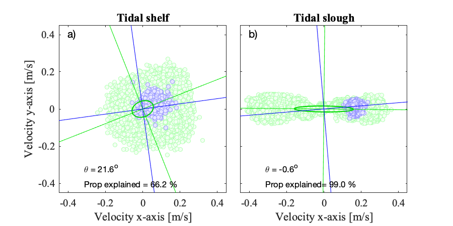
[[File:Frame of reference adv.png|600px|frame|Fig 1. Examples of measured velocities from two ADVs highlighting that their x-axis may be un-aligned with the flow's. The blue dots and lines that represent the principal axes are for a 5-min subset of the entire timeseries shown in red. The left example (a) is from the shelf break in ~190 m of water, while the right example (b) is from a tidally-influenced slough (a few meters deep). The statistics in each panel were estimated for the entire timeseries, and highlights that the flow's frame of reference is much more variable in the Tidal shelf example (a) than the Tidal Slough (b). Another key difference is that in the slough example (b), the instrument's x-axis was oriented along the length of the channel, and thus in the general direction of the flow. This is the ideal set-up for turbulence measurements from acoustic-Doppler velocity-meters.]] | |||
In some setups, the instrument's x-axis is already aligned with the general direction of the mean flow. This is particularly desirable when planning on calculating turbulent shear stresses via covariances as correlated noise may ensue when rotating the measurements into a new frame of reference ({{FontColor|fg=red|text=Insert reference}}). For some shallow systems, it's possible to align an instrument's x-axis with the direction of the flow (see Fig 1b). Alternatively, the entire dataset may be rotated using the velocities' principal components over the entire timeseries. For instance, the Tidal Slough example (Fig 1a) flows generally along the channel's length except at the turn of the tide. In other datasets, like the Tidal Shelf, it's necessary to rotate each segment into the flow's direction. | |||
Revision as of 15:16, 8 March 2022
{{#default_form:Processing}}
{{#arraymap:
Velocity point-measurements
|,|x||}}
{{#arraymap:level 2 segmented and quality controlled|,|x||}}
The velocities are measured in either the instrument's coordinate system (XYZ), beam coordinates, or more rarely in the earth's coordinate system (ENU=east, north and up). When estimating , measured velocities are often rotated in the flow's frame of reference since inertial subrange model differs between the velocity components, and the effects of anisotropy are more pronounced in the transverse and vertical direction. When the vertical velocities are too heavily impacted by anisotropy, the longitudinal direction may be used to derive . In these instances, the longitudinal velocity must align with the mean flow direction, which may require rotating the measurements into a new frame of reference i.e., the analysis frame of reference.

In some setups, the instrument's x-axis is already aligned with the general direction of the mean flow. This is particularly desirable when planning on calculating turbulent shear stresses via covariances as correlated noise may ensue when rotating the measurements into a new frame of reference (Insert reference). For some shallow systems, it's possible to align an instrument's x-axis with the direction of the flow (see Fig 1b). Alternatively, the entire dataset may be rotated using the velocities' principal components over the entire timeseries. For instance, the Tidal Slough example (Fig 1a) flows generally along the channel's length except at the turn of the tide. In other datasets, like the Tidal Shelf, it's necessary to rotate each segment into the flow's direction.
