Example forward-difference

Consider the example of an ADCP with a beam angle of $20^{\circ }$, configured with a vertical bin size of 10 cm, recording profiles at 1 second intervals with a data segment length of 300 seconds. The Level 1 QC of the data identified that good data was typically returned from bins 1 to 30.

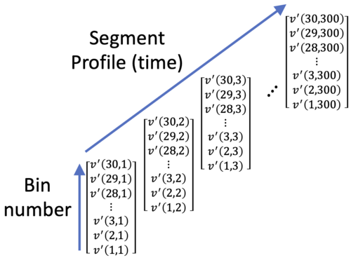
The velocity data from a single beam for a single data segment can therefore be visualised as:

The square of the velocity difference between bins separated by $\delta$ bins is then evaluated for each $t$. So for $t_1$, bin 1 and $\delta =1$, we get:

$\mathrm{\Delta }v(1,1,1)={[v^{\prime }(1,1)-v^{\prime }(2,1)]}^2$

For bin 1 the squared velocity difference can be evaluated for $1⩽\delta ⩽29$, whilst for bin 2 it is restricted to $1⩽\delta ⩽28$, reducing by 1 with each bin, so that for bin 29, it can only be evaluated for $\delta =1$ and there are no options for bin 30. This is summarised as follows:

The mean is then taken across the 300 profiles in the data segment e.g.

$D(1,1)=\sum _{t=1}^{300}D(1,\delta ,t)$

Return to Forward-difference