Nasmyth spectrum
| Short definition of Nasmyth spectrum |
|---|
| Nasmyth shear spectrum |
This is the common definition for Nasmyth spectrum, but other definitions maybe discussed within the wiki.
Nasmyth shear spectrum
There is no theoretical derivation for the spectrum of velocity that encompasses the inertial subrange and the range that is affected by viscosity (the dissipation range). Such a spectrum would be a gauge for judging the quality of a measured spectrum. There are only empirical spectra based on the average of many observations. The earliest of these is the Nasmyth spectrum[1] that was later tabulated by Oakey (1982)[2]. The data were collected in a tidal channel using a hot-film anemometer that measures the fluctuations of velocity in the direction of profiling.
That is, Nasmyth measured [math]\displaystyle{ E_{11}(k_1) }[/math]. His spectra were non-dimensionalized to form [math]\displaystyle{ F_{11} }[/math] and these spectra were averaged into 15 wavenumber bins that are spread fairly uniformly in logarithmic space (Table 1). Oakey used the isotropic relationship to derive the spectrum of the cross-stream component of velocity, [math]\displaystyle{ F_{22}(\hat{k}_1) }[/math], and hence, the universal shear spectrum [math]\displaystyle{ G_{22}(\hat{k}_1)=(2\pi \hat{k}_1)^2F_{22}(\hat{k}_1) }[/math].
Nasmyth shear spectrum -- [math]\displaystyle{ 1^{\mathrm{st}} }[/math] approximation

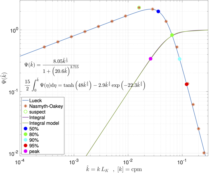
Wolk et al (2002)[3] provided a simple mathematical model for the Nasmyth spectrum predicated on the assumption that the eighth spectral point is erroneous (Figure 2). This model is
[math]\displaystyle{ \Psi_{N_1} (\hat{k}_1)= \frac{8.05\,\hat{k}_1^{1/3}}{1+ \left(20.6\,\hat{k}_1\right)^{3.715}} }[/math]
and the model for the integral of this spectrum is
[math]\displaystyle{ I_{N_1}(\hat{k}_1) = \frac{15}{2} \int_0^{\hat{k}_1} \Psi_{N_1} (\xi) \mathrm{d}\xi = \tanh\left(48\,\hat{k}_1^{4/3}\right) - 2.9\,\hat{k}_1^{4/3} \exp\left(-22.3\, \hat{k}_1^{4/3} \right) }[/math]
The one-dimensional Kolmogorov constant of this model is
[math]\displaystyle{ C_1=\frac{3}{4} \frac{8.05}{(2\pi)^{4/3}}=0.52 }[/math]
| [math]\displaystyle{ k_1 L_K }[/math] | [math]\displaystyle{ F_{11}(k_1L_K) }[/math] | [math]\displaystyle{ \Psi_N(k_1L_K) }[/math] |
|---|---|---|
| [math]\displaystyle{ 2.830\times 10^{-4} }[/math] | [math]\displaystyle{ 1.254\times 10^{5} }[/math] | [math]\displaystyle{ 0.5285 }[/math] |
| [math]\displaystyle{ 5.0303\times 10^{-4} }[/math] | [math]\displaystyle{ 4.799\times 10^{4} }[/math] | [math]\displaystyle{ 0.6397 }[/math] |
| [math]\displaystyle{ 8.950\times 10^{-4} }[/math] | [math]\displaystyle{ 1.842\times 10^{4} }[/math] | [math]\displaystyle{ 0.7763 }[/math] |
| [math]\displaystyle{ 1.592\times 10^{-3} }[/math] | [math]\displaystyle{ 7.050\times 10^{3} }[/math] | [math]\displaystyle{ 0.9404 }[/math] |
| [math]\displaystyle{ 2.830\times 10^{-3} }[/math] | [math]\displaystyle{ 2.699\times 10^{3} }[/math] | [math]\displaystyle{ 1.138 }[/math] |
| [math]\displaystyle{ 5.0323\times 10^{-3} }[/math] | [math]\displaystyle{ 1.036\times 10^{3} }[/math] | [math]\displaystyle{ 1.380 }[/math] |
| [math]\displaystyle{ 8.950\times 10^{-3} }[/math] | [math]\displaystyle{ 3.964\times 10^{2} }[/math] | [math]\displaystyle{ 1.682 }[/math] |
| [math]\displaystyle{ 1.592\times 10^{-2} }[/math] | [math]\displaystyle{ 1.490\times 10^{2} }[/math] | [math]\displaystyle{ 2.302 }[/math] |
| [math]\displaystyle{ 2.830\times 10^{-2} }[/math] | [math]\displaystyle{ 3.574\times 10^{1} }[/math] | [math]\displaystyle{ 2.176 }[/math] |
| [math]\displaystyle{ 5.0330\times 10^{-2} }[/math] | [math]\displaystyle{ 5.600\times 10^{0} }[/math] | [math]\displaystyle{ 1.373 }[/math] |
| [math]\displaystyle{ 7.977\times 10^{-2} }[/math] | [math]\displaystyle{ 7.214\times 10^{-1} }[/math] | [math]\displaystyle{ 0.5278 }[/math] |
| [math]\displaystyle{ 1.264\times 10^{-1} }[/math] | [math]\displaystyle{ 6.580\times 10^{-2} }[/math] | [math]\displaystyle{ 0.1342 }[/math] |
| [math]\displaystyle{ 1.592\times 10^{-1} }[/math] | [math]\displaystyle{ 1.812\times 10^{-2} }[/math] | [math]\displaystyle{ 0.0616 }[/math] |
| [math]\displaystyle{ 2.004\times 10^{-1} }[/math] | [math]\displaystyle{ 4.552\times 10^{-3} }[/math] | [math]\displaystyle{ 0.0249 }[/math] |
| [math]\displaystyle{ 2.522\times 10^{-1} }[/math] | [math]\displaystyle{ 1.197\times 10^{-3} }[/math] | [math]\displaystyle{ 0.0101 }[/math] |
Table 1. The Nasmyth non-dimensional velocity and shear spectrum after Oakey (1982)[2]. The one-dimensional wavenumber is in units of [math]\displaystyle{ \mathrm{cpm} }[/math] and is non-dimensionalized by the Kolmogorov length, [math]\displaystyle{ L_K }[/math].
Nasmyth shear spectrum -- [math]\displaystyle{ 2^{\mathrm{nd}} }[/math] approximation
The notion that the eighth value of the Nasmyth spectrum is erroneous may be a false one. Observations of all three velocity components in a high Reynolds number wind tunnel by Saddoughi and Veeravalli (1994)[4] indicate that all three components have a spectral rise above the [math]\displaystyle{ k_1^{1/3} }[/math] tendency of the inertial subrange, shortly before the spectrum falls rapidly due to viscosity, and that the rise is larger in the shear than in the strain components (see Figure 13 of Saddoughi and Veeravalli, 1994[4]). However, the rise seen in the Nasmyth shear spectrum is not evident in the Nasmyth strain spectrum [math]\displaystyle{ G_{11} }[/math].


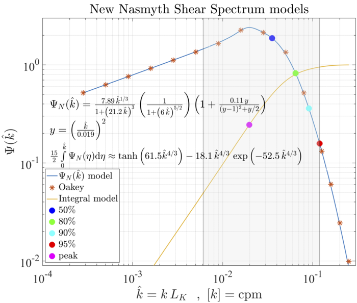
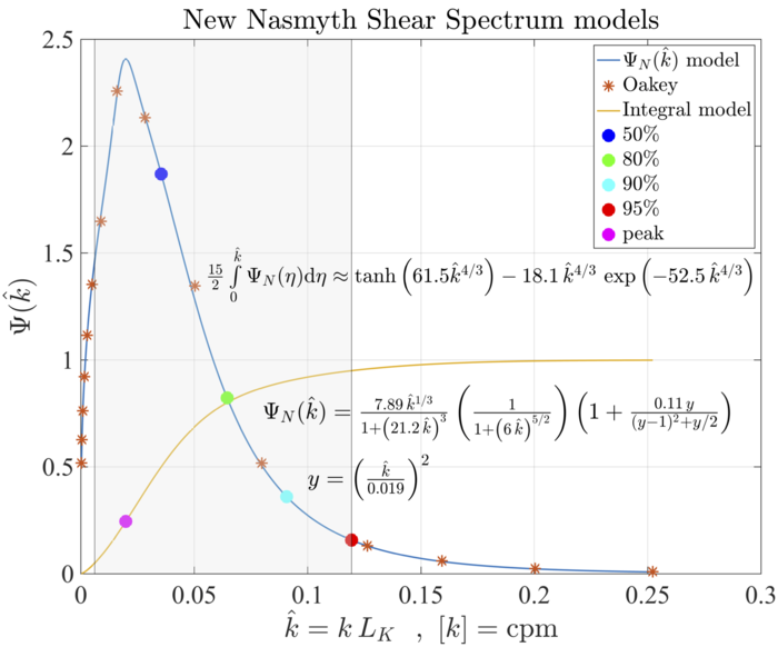
Lueck (2021b)[5] re-examined the spectrum tabulated by Oakey (1982)[2] and noticed that the strain spectrum, [math]\displaystyle{ \left(2\pi \hat{k}_1\right)^2 F_{11} }[/math] integrates to a value that is [math]\displaystyle{ 2\% }[/math] higher than [math]\displaystyle{ 1/15 }[/math]. Therefore, the tabulated values for [math]\displaystyle{ F_{11} }[/math] should be reduced by this factor. A second model that takes into account the spectral rise displayed by the eighth point, and uses the reduced values for [math]\displaystyle{ F_{11} }[/math], is
[math]\displaystyle{ \begin{equation} \begin{split} \Psi_{N_2}(\hat{k}_1) &= \left(\frac{7.89\,\hat{k}_1^{1/3}}{1+ \left(21.2\,\hat{k}_1 \right)^3 }\right) \left( \frac{1}{1+ \left(6\,\hat{k}_1\right)^{5/2} }\right) \left(1+ \frac{0.11 y}{(y-1)^2 + y/2} \right) \\ y &= \left(\frac{\hat{k}_1}{0.019}\right)^2 \end{split} \end{equation} }[/math]
which integrates to a value that is only [math]\displaystyle{ 0.1\% }[/math] larger than [math]\displaystyle{ 15/2 }[/math][5]. The one-dimensional Kolmogorov constant is [math]\displaystyle{ C_1=0.51 }[/math] for this model. An approximation for the integral of this spectrum is
[math]\displaystyle{ I_{N_2}(\hat{k}_1) = \frac{15}{2} \int_0^{\hat{k}_1} \Psi_{N_2} (\xi)\,\mathrm{d}\xi = \tanh\left(61.5\,\hat{k}_1^{4/3}\right) - 18.1\,\hat{k}_1^{4/3} \exp\left(-52.5\,\hat{k}_1^{4/3}\right) }[/math]
This approximation is shown in log-log space in Figure 3, and in linear space in Figure 4.
References
- ↑ Nasmyth, P. W. (1970). Ocean turbulence (Ph. D. Thesis). University of British Columbia.
- ↑ Jump up to: 2.0 2.1 2.2 2.3 Oakey, N. S. (1982). Determination of the rate of dissipation of turbulent energy from simultaneous temperature and velocity shear microstructure measurements. Journal of Physical Oceanography, 12(3), 256-271.
- ↑ Wolk, F., Yamazaki, H., Seuront, L., & Lueck, R. G. (2002). A new free-fall profiler for measuring biophysical microstructure. Journal of Atmospheric and Oceanic Technology, 19(5), 780-793.
- ↑ Jump up to: 4.0 4.1 Saddoughi, S. G., & Veeravalli, S. V. (1994). Local isotropy in turbulent boundary layers at high Reynolds number. Journal of Fluid Mechanics, 268, 333-372.
- ↑ Jump up to: 5.0 5.1 Lueck, R. G., 2021b: The statistics of oceanic turbulence measurements: Shear variance and dissipation rates. J. Phys. Oceanogr.,–, submitted, doi:--.
