Processing your ADCP data using structure function techniques

To calculate the dissipation rate at a specific range bin and a specific time ensemble:

Schematic showing along-beam distance [math]\displaystyle{ r }[/math] and radial velocities.

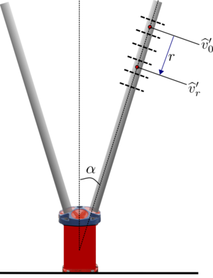
1. Extract or compute the along-beam bin center separation [[math]\displaystyle{ \delta r_0 }[/math]] based on the instrument geometry
2. Calculate the along-beam velocity fluctuation time-series in each bin [math]\displaystyle{ n }[/math], where [[math]\displaystyle{ b’(n, t_s) }[/math]] from the along-beam velocity data that has met the QC criteria (i.e. the data in Level 2 of the netcdf file). Note [math]\displaystyle{ t_s }[/math] is the timeseries index within a segment.
3. Select the maximum distance ([math]\displaystyle{ r_{max} }[/math]) over which to compute the structure function based on conditions of the flow (e.g., expected max overturn, spectral range corresponding to [math]\displaystyle{ k^{-5/3} }[/math]). The corresponding number of bins is [[math]\displaystyle{ n_{\text{rmax}} = r_{max} / \delta r_0 }[/math]]
4. Calculate the structure function [math]\displaystyle{ D_{ll} }[/math] for all possible bin separations [math]\displaystyle{ \delta }[/math] within [math]\displaystyle{ r_{max} }[/math] using either a bin-centred difference scheme or a forward-difference scheme.
5. Perform a regression of [math]\displaystyle{ D_{ll}(n,\delta) }[/math] against [math]\displaystyle{ (\delta r)^{2/3} }[/math] for the appropriate range of bins and [math]\displaystyle{ \delta }[/math]r separation distances. Be aware of special considerations for forward-difference, center-difference schemes in setting up the regression calculation. The regression is typically done as a least-squares fit, either as:
   
   [math]\displaystyle{ D_{ll} = a_0 + a_1 (\delta r)^{2/3} }[/math];

or as

[math]\displaystyle{ D_{ll} = a_0 + a_1 (\delta r)^{2/3}+a_3((\delta r)^{2/3})^3 }[/math]

the former being the canonical method that excludes non-turbulent velocity differences between bins, whereas the latter is a modified method that includes non-turbulent velocity differences between bins due to any oscillatory signal (e.g. surface waves, motion of the ADCP on a mooring).

6. Use the coefficient [math]\displaystyle{ a_1 }[/math] to calculate [math]\displaystyle{ \varepsilon }[/math] as
   
   [math]\displaystyle{ \varepsilon = \left(\frac{a_1}{C_2}\right)^{2/3} }[/math]
   
   where [math]\displaystyle{ C_2 }[/math] is an empirical constant, typically taken as 2.0 or 2.1.

---

Next step: Apply quality-control on dissipation rates (QA2)

Previous step: Apply quality-control on velocity time series data (QA1)

Return to ADCP Flow Chart front page