Decomposing velocity measurements: Difference between revisions
| (8 intermediate revisions by the same user not shown) | |||
| Line 4: | Line 4: | ||
}} | }} | ||
The quality-controlled velocities can be [[Detrending time series|detrended]] before being further analysed to determine [[Velocity past the sensor|mean flow past the sensor]] and [[Surface wave statistics|surface wave statistics]]. These quantities | The quality-controlled velocities can be [[Detrending time series|detrended]] before being further analysed to determine [[Velocity past the sensor|mean flow past the sensor]] and [[Surface wave statistics|surface wave statistics]]. These quantities are necessary for later choosing the appropriate [[Velocity inertial subrange model| inertial subrange model]] for [[Spectral fitting|spectral fitting]]. | ||
Quality-controlled velocities may also need detrended before applying various [[Velocity despiking|despiking]]. | Quality-controlled velocities may also need to be detrended before applying various [[Velocity despiking|despiking]]. Because estimating <math>\varepsilon</math> is done from the spectral observations, the analysis is insensitive to this step provided that we don’t filter out the scales shorter than the [[Segmenting datasets| segment length]]. | ||
<div><ul> | |||
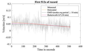
<li style="display: inline-block; vertical-align: top;"> [[File:Short timeseries.png|thumb|none|350px|512 s segment of the measured velocities after applying different [[Detrending time series|detrending methods]]]] | |||
</li> | |||
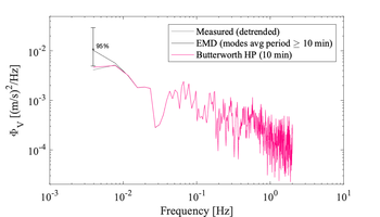
<li style="display: inline-block; vertical-align: top;"> [[File:Short_spectra.png|thumb|none|350px|Example velocity spectra of the short 512 s of records before and after different detrending techniques applied to the original 6h time series. The impact of the detrending method can be seen at the lowest frequencies only]] </li> | |||
</ul></div> | |||
---- | ---- | ||
Return to [[ | Return to [[Preparing quality-controlled velocities]] | ||
Latest revision as of 19:08, 5 July 2022
{{#default_form:Processing}}
{{#arraymap:
Velocity point-measurements
|,|x||}}
{{#arraymap:level 2 segmented and quality controlled|,|x||}}
The quality-controlled velocities can be detrended before being further analysed to determine mean flow past the sensor and surface wave statistics. These quantities are necessary for later choosing the appropriate inertial subrange model for spectral fitting.
Quality-controlled velocities may also need to be detrended before applying various despiking. Because estimating <math>\varepsilon</math> is done from the spectral observations, the analysis is insensitive to this step provided that we don’t filter out the scales shorter than the segment length.
-

512 s segment of the measured velocities after applying different detrending methods -

Example velocity spectra of the short 512 s of records before and after different detrending techniques applied to the original 6h time series. The impact of the detrending method can be seen at the lowest frequencies only
Return to Preparing quality-controlled velocities
