Velocity despiking: Difference between revisions
No edit summary |
|||
| (47 intermediate revisions by the same user not shown) | |||
| Line 3: | Line 3: | ||
|level=level 1 raw | |level=level 1 raw | ||
}} | }} | ||
=Overview = | =Overview = | ||
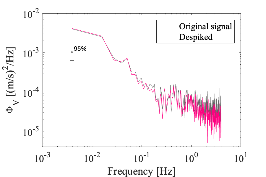
Any measured signal may be contaminated by spikes. These spikes are typically short-lived and transient, which result in | Any measured signal may be contaminated by spikes. These spikes are typically short-lived and transient, which result in sudden change in the [[Media:Velocities spike.png| measured velocities]]. These spikes must be removed because they can alter quite dramatically the [[Media:Despike spectra.png|velocity spectra]], which is then used for fitting [[Velocity inertial subrange model|inertial subrange model]]. | ||
This category of methods is quite common in the literature and has been reviewed extensively by others <ref name="GoringNikora"/><ref name="Starkenburg"/>. These methods compare the original signal against a smoothed version, and values exceeding a threshold are deemed spikes. Most commonly, the threshold is applied to the time series of [[Media:Smoothed velocities.png|velocity differences]] obtained by subtracting the smoothed velocities from the original spiky signal. | |||
<div><ul> | <div><ul> | ||
<li style="display: inline-block; vertical-align: top;"> [[File:Velocities spike.png|thumb|none| | <li style="display: inline-block; vertical-align: top;"> [[File:Velocities spike.png|thumb|none|350px|Example velocities measured by an [[Acoustic-Doppler Velocimeters| acoustic-Doppler velocimeters]]]] </li> | ||
<li style="display: inline-block; vertical-align: top;"> [[File:Despike spectra.png|thumb|none| | <li style="display: inline-block; vertical-align: top;"> [[File:Despike spectra.png|thumb|none|350px|Example velocity spectra before and after removing spikes. The variance of the despiked signal has reduced by 12% even though there were 30 spikes]] </li> | ||
</ul></div> | </ul></div> | ||
Spikes in velocities measured by [[Acoustic-Doppler Velocimeters| acoustic-Doppler velocimeters]] can result from aliasing of the Doppler signal, in particular when pulses become contaminated by reflecting from complex objects and boundaries <ref name="GoringNikora">{{Cite journal|authors= D. G. Goring and V.I. Nikora|journal_or_publisher= Journal of Hydraulic Engineering|paper_or_booktitle= Despiking Acoustic Doppler Velocimeter Data | |||
|year= 2002|doi= 10.1061/ASCE0733-94292002128:1117}}</ref>. Several techniques exist for despiking. The methods of Goring and Nikora<ref name="GoringNikora" /> was developed specifically for acoustic-doppler velocity measurements. The JTECH paper by Starkenburg et al. (2016)<ref name="Starkenburg">{{Cite journal|authors= D. Starkenburg, S. Metzger, G.J. Fochesatto, J.G Alfieri, R. Gens, A. Prakash and J. Cristobal|journal_or_publisher= J. Atmos. Oceanic Technoly|paper_or_booktitle= Assessment of Despiking Methods for Turbulence Data in Micrometeorology | |||
|year= 2016|doi= 10.1175/JTECH-D-15-0154.1}}</ref> review a number of methods for atmospheric turbulence measurements such as eddy-correlation flux estimates, including those of Goring and Nikora. Starkenburg et al. (2016) deemed median-based filtering a more robust means of filtering data since it can handle missing points more easily, and handles better time series with evidence of low-frequency coherent turbulent structures. | |||
The subgroup has recommended the use of the median filter despiking technique <ref name="Brock">{{Cite journal|authors=F.V. Brock|journal_or_publisher= J. Atmos. Oceanic Technoly|paper_or_booktitle= A nonlinear filter to remove impulse noise from meteorological data | |||
|year= 1986|doi= 10.1175/1520-0426(1986)003,0051:ANFTRI.2.0.CO;2}}</ref>. | |||
= Application of the median-filter = | |||
In the 1970s, scientists developed methods based on nonlinear median filters | In the 1970s, scientists developed methods based on nonlinear median filters | ||
<ref>{{Cite journal|authors=A.E. Beaton, J.W. Tukey|journal_or_publisher= Technometrics|paper_or_booktitle= The fitting of power series, meaning polynomials, illustrated on band-spectroscopic data | <ref>{{Cite journal|authors=A.E. Beaton, J.W. Tukey|journal_or_publisher= Technometrics|paper_or_booktitle= The fitting of power series, meaning polynomials, illustrated on band-spectroscopic data | ||
|year= 1974|doi=10.1080/00401706.1974.10489171}}</ref>. | |year= 1974|doi=10.1080/00401706.1974.10489171}}</ref>. These filters are less biased by spikes than other linear operations such as low-pass Butterworth filters<ref name="Starkenburg"/>. The moving median filter, for example, only requires a window length, i.e, the number of points over which to calculate the median. This window length must be longer than the duration of spikes, which can span consecutive samples. This number must also be sufficiently short to compute a reasonable local median (see Table 1 of Starkenburg et al 2016<ref name="Starkenburg"/>). The challenge then becomes determining the threshold for identifying spikes. | ||
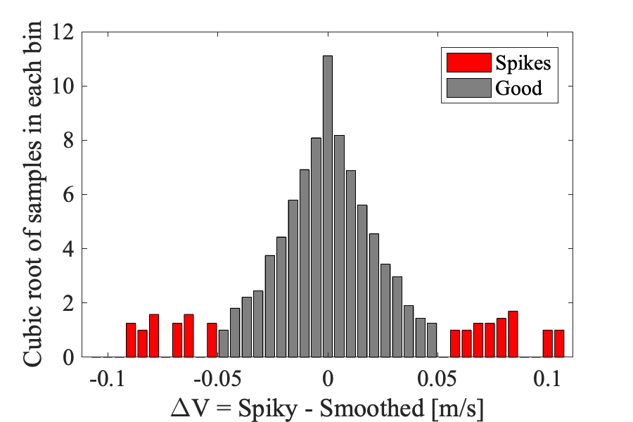
Some filter-based methods use thresholds based on a factor of the original time series' standard deviation (e.g., Tukey method discussed by Goring & Nikora<ref name="GoringNikora" />). The results of the analysis then become sensitive to this choice of factor. A more automated means to identify the threshold was proposed by Brock (1986)<ref name="Brock" /> using a [[Media:Threshold logic Brock1986.png|histogram of velocity differences]] (the original minus the smoothed signal). The local minimums on either side from the center define the positive and negative thresholds. Velocity differences exceeding these thresholds are deemed to be spikes.[[File:Threshold logic Brock1986.png|400px|thumb|Histogram of velocity differences between the original (spiky) and smoothed signals. The local minimum denotes the lower and upper thresholds for identifying spikes. The standard deviation of the original time series is 2 cm/s, while the thresholds are -4.8 and 5.3 cm/s.]] | |||
=Notes= | =Notes= | ||
Latest revision as of 21:14, 9 September 2026
Overview
Any measured signal may be contaminated by spikes. These spikes are typically short-lived and transient, which result in sudden change in the measured velocities. These spikes must be removed because they can alter quite dramatically the velocity spectra, which is then used for fitting inertial subrange model.
This category of methods is quite common in the literature and has been reviewed extensively by others [1][2]. These methods compare the original signal against a smoothed version, and values exceeding a threshold are deemed spikes. Most commonly, the threshold is applied to the time series of velocity differences obtained by subtracting the smoothed velocities from the original spiky signal.
-
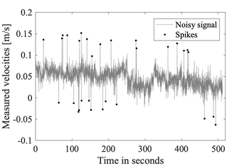
Example velocities measured by an acoustic-Doppler velocimeters -
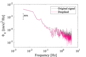
Example velocity spectra before and after removing spikes. The variance of the despiked signal has reduced by 12% even though there were 30 spikes


Spikes in velocities measured by acoustic-Doppler velocimeters can result from aliasing of the Doppler signal, in particular when pulses become contaminated by reflecting from complex objects and boundaries [1]. Several techniques exist for despiking. The methods of Goring and Nikora[1] was developed specifically for acoustic-doppler velocity measurements. The JTECH paper by Starkenburg et al. (2016)[2] review a number of methods for atmospheric turbulence measurements such as eddy-correlation flux estimates, including those of Goring and Nikora. Starkenburg et al. (2016) deemed median-based filtering a more robust means of filtering data since it can handle missing points more easily, and handles better time series with evidence of low-frequency coherent turbulent structures.
The subgroup has recommended the use of the median filter despiking technique [3].
Application of the median-filter
In the 1970s, scientists developed methods based on nonlinear median filters [4]. These filters are less biased by spikes than other linear operations such as low-pass Butterworth filters[2]. The moving median filter, for example, only requires a window length, i.e, the number of points over which to calculate the median. This window length must be longer than the duration of spikes, which can span consecutive samples. This number must also be sufficiently short to compute a reasonable local median (see Table 1 of Starkenburg et al 2016[2]). The challenge then becomes determining the threshold for identifying spikes.
Some filter-based methods use thresholds based on a factor of the original time series' standard deviation (e.g., Tukey method discussed by Goring & Nikora[1]). The results of the analysis then become sensitive to this choice of factor. A more automated means to identify the threshold was proposed by Brock (1986)[3] using a histogram of velocity differences (the original minus the smoothed signal). The local minimums on either side from the center define the positive and negative thresholds. Velocity differences exceeding these thresholds are deemed to be spikes.

Notes
- ↑ 1.0 1.1 1.2 1.3 D. G. Goring and V.I. Nikora. 2002. Despiking Acoustic Doppler Velocimeter Data. Journal of Hydraulic Engineering. doi:10.1061/ASCE0733-94292002128:1117
- ↑ 2.0 2.1 2.2 2.3 D. Starkenburg, S. Metzger, G.J. Fochesatto, J.G Alfieri, R. Gens, A. Prakash and J. Cristobal. 2016. Assessment of Despiking Methods for Turbulence Data in Micrometeorology. J. Atmos. Oceanic Technoly. doi:10.1175/JTECH-D-15-0154.1
- ↑ 3.0 3.1 F.V. Brock. 1986. A nonlinear filter to remove impulse noise from meteorological data. J. Atmos. Oceanic Technoly. doi:10.1175/1520-0426(1986)003,0051:ANFTRI.2.0.CO;2
- ↑ A.E. Beaton, J.W. Tukey. 1974. The fitting of power series, meaning polynomials, illustrated on band-spectroscopic data. Technometrics. doi:10.1080/00401706.1974.10489171