Processing your ADCP data using structure function techniques: Difference between revisions
From Atomix
Yuengdjern (talk | contribs) No edit summary |
Yuengdjern (talk | contribs) No edit summary |
||
| (55 intermediate revisions by 5 users not shown) | |||
| Line 1: | Line 1: | ||
To calculate the dissipation rate at a specific range bin and a specific time ensemble: | |||
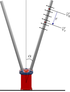
# Extract or compute the along-beam | [[File:ADCPschematic SF.png|thumb|Schematic showing along-beam distance <math> r </math> and radial velocities. ]] | ||
# Calculate the along-beam velocity | |||
# Extract or compute the [[along-beam bin center separation]] [<math>\delta r_0</math>] based on the instrument geometry | |||
# Calculate the [[along-beam velocity fluctuation]] time-series in each bin <math>n</math>, where [<math>b’(n, t_s)</math>] from the along-beam velocity data that has met the QC criteria (i.e. the data in Level 2 of the netcdf file). Note <math> t_s </math> is the timeseries index within a segment. | |||
# Select the maximum distance (<math>r_{max}</math>) over which to compute the structure function based on conditions of the flow (e.g., expected max overturn, spectral range corresponding to <math> k^{-5/3} </math>). The corresponding number of bins is [<math>n_{\text{rmax}} = r_{max} / \delta r_0</math>] | |||
# Calculate the structure function <math>D_{ll}</math> for all possible bin separations <math>\delta</math> within <math>r_{max}</math> using either a [[bin-centred difference scheme]] or a [[forward-difference]] scheme. | |||
# Perform a regression of <math>D_{ll}(n,\delta)</math> against <math>(\delta r)^{2/3}</math> for the appropriate range of bins and <math>\delta</math>r</sub> separation distances. Be aware of [[Regressing structure function against bin separation | special considerations for forward-difference, center-difference schemes]] in setting up the regression calculation. The regression is typically done as a least-squares fit, either as: <br /><br /> <math>D_{ll} = a_0 + a_1 (\delta r)^{2/3}</math>; | |||
:: or as | |||
# Select the maximum distance over which to compute the structure function based on conditions of the flow (e.g., expected max overturn) [ | :: <math>D_{ll} = a_0 + a_1 (\delta r)^{2/3}+a_3((\delta r)^{2/3})^3 </math> <br /><br /> the former being the [[canonical structure function method | canonical method]] that excludes non-turbulent velocity differences between bins, whereas the latter is a [[modified structure function method | modified method]] that includes non-turbulent velocity differences between bins due to any oscillatory signal (e.g. surface waves, motion of the ADCP on a mooring). | ||
# | <ol type="1" start=6> | ||
# | <li> Use the coefficient <math>a_1</math> to calculate <math>\varepsilon</math> as <br /><br /> <math>\varepsilon = \left(\frac{a_1}{C_2}\right)^{2/3}</math> <br /><br /> where <math>C_2</math> is an [[ Structure function empirical constant | empirical constant]], typically taken as 2.0 or 2.1. | ||
</ol> | |||
---- | |||
Next step: [[Final data review (QA2) | Apply quality-control on dissipation rates (QA2)]] <br></br> | |||
Previous step:[[Raw data review (QA1) | Apply quality-control on velocity time series data (QA1)]]<br></br> | |||
Return to [[ADCP structure function flow chart| ADCP Flow Chart front page]] | |||
[[Category:Velocity profilers]] | |||
Latest revision as of 15:51, 30 May 2022
To calculate the dissipation rate at a specific range bin and a specific time ensemble:

- Extract or compute the along-beam bin center separation [<math>\delta r_0</math>] based on the instrument geometry
- Calculate the along-beam velocity fluctuation time-series in each bin <math>n</math>, where [<math>b’(n, t_s)</math>] from the along-beam velocity data that has met the QC criteria (i.e. the data in Level 2 of the netcdf file). Note <math> t_s </math> is the timeseries index within a segment.
- Select the maximum distance (<math>r_{max}</math>) over which to compute the structure function based on conditions of the flow (e.g., expected max overturn, spectral range corresponding to <math> k^{-5/3} </math>). The corresponding number of bins is [<math>n_{\text{rmax}} = r_{max} / \delta r_0</math>]
- Calculate the structure function <math>D_{ll}</math> for all possible bin separations <math>\delta</math> within <math>r_{max}</math> using either a bin-centred difference scheme or a forward-difference scheme.
- Perform a regression of <math>D_{ll}(n,\delta)</math> against <math>(\delta r)^{2/3}</math> for the appropriate range of bins and <math>\delta</math>r separation distances. Be aware of special considerations for forward-difference, center-difference schemes in setting up the regression calculation. The regression is typically done as a least-squares fit, either as:
<math>D_{ll} = a_0 + a_1 (\delta r)^{2/3}</math>;
- or as
- <math>D_{ll} = a_0 + a_1 (\delta r)^{2/3}+a_3((\delta r)^{2/3})^3 </math>
the former being the canonical method that excludes non-turbulent velocity differences between bins, whereas the latter is a modified method that includes non-turbulent velocity differences between bins due to any oscillatory signal (e.g. surface waves, motion of the ADCP on a mooring).
- Use the coefficient <math>a_1</math> to calculate <math>\varepsilon</math> as
<math>\varepsilon = \left(\frac{a_1}{C_2}\right)^{2/3}</math>
where <math>C_2</math> is an empirical constant, typically taken as 2.0 or 2.1.
Next step: Apply quality-control on dissipation rates (QA2)
Previous step: Apply quality-control on velocity time series data (QA1)
Return to ADCP Flow Chart front page
