Segmenting datasets

Once the raw observations have been quality-controlled, then you must split the time series into shorter segments by considering:

• Time and length scales of turbulence
• Stationarity of the segment and Taylor's frozen turbulence hypothesis
• Statistical significance of the resulting spectra

Considerations

Measurements are typically collected in the following two ways:

• continuously, or in such long bursts that they can be considered continuous
• short bursts that are typically at most 2-3x the expected largest turbulence time scales (e.g., 10 min in ocean environments)

This segmenting step dictates the minimum burst duration when setting up your equipment. The act of chopping a time series into smaller subsets, i.e., segments, is effectively a form of low-pass (box-car) filtering. How to segment the time series is usually a more important consideration than detrending the time series since estimating $\epsilon$ relies on resolving the inertial subrange in the final spectra computed over each segment.

• 

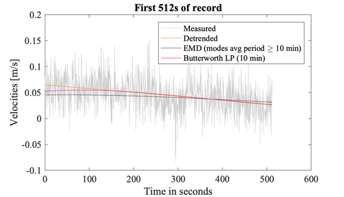
  512 s segment of the measured velocities after applying different detrending methods

• 

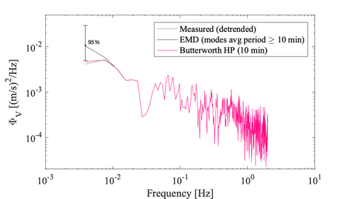
  Example velocity spectra of the short 512 s of records before and after different detrending techniques applied to the original 6h time series. The impact of the detrending method can be seen at the lowest frequencies only

Trade-offs

The shorter the segment, the higher the temporal resolution of the final $\epsilon$ time series and the more likely the segment will be stationary. However, the spectrum's lowest resolved frequency and frequency resolution depends on the duration of the signal used to construct the spectrum. Therefore, the segment must remain sufficiently long such that the lowest wavenumber (frequencies) of the inertial subrange are retained by the spectra. This is particularly important when measurement noise drowns the highest wavenumber (frequencies) of the inertial subrange. Thus, using too short segments may inadvertently render the resulting spectra unusable for deriving $\epsilon$ from the inertial subrange by virtue of no longer resolving this subrange.

Recommendations

A good rule of thumb for tidally-influenced environments is 5 to 15 min segments, but this may be shorter in certain energetic and fast-moving flows. include example data in plot highlighting low and high epsilon, and different speeds leading to much shorter and longer segmenting periods

Example theoretical velocity spectra for different $\epsilon$ with the empirical limit $\hat{k}{L}_k\sim 0.1$ denoted by the diamonds ($\hat{k}$ is in rad/m). The inertial subrange extends to smaller wavenumber $k$ [cpm] as $\epsilon$ increases. The lowest frequency resolved by a spectra depends on the fft-length used when computing the spectra. The colored lines are spectral observations from a dataset with fast speeds and large $\epsilon$, allowing the use of relatively short segments (128s) to estimate the spectra from fft-length of 32 s (2048 samples @ 64 Hz). The impact of turbulence anisotropy is also visible through the flattening of the spectra around 1 cpm

Notes

---

Return to Preparing_quality-controlled_velocities