Segmenting datasets: Difference between revisions
From Atomix
mNo edit summary |
|||
| Line 17: | Line 17: | ||
* continuously, or in such long bursts that they can be considered continuous | * continuously, or in such long bursts that they can be considered continuous | ||
* short bursts that are typically at most 2-3x the expected largest [[Time and length scales of turbulence|turbulence time scales]] (e.g., 10 min in ocean environments) | * short bursts that are typically at most 2-3x the expected largest [[Time and length scales of turbulence|turbulence time scales]] (e.g., 10 min in ocean environments) | ||
This segmenting step dictates the minimum burst duration when setting up your equipment. The act of chopping a time series into smaller subsets, i.e., segments, is effectively a form of low-pass (box-car) filtering. How to [[Segmenting datasets|segment]] the time series is usually a more important consideration than [[Detrending time series|detrending the time series]] since estimating <math>\varepsilon</math> relies on resolving the [[Velocity inertial subrange|inertial subrange]]. | This segmenting step dictates the minimum burst duration when setting up your equipment. The act of chopping a time series into smaller subsets, i.e., segments, is effectively a form of low-pass (box-car) filtering. How to [[Segmenting datasets|segment]] the time series is usually a more important consideration than [[Detrending time series|detrending the time series]] since estimating <math>\varepsilon</math> relies on resolving the [[Velocity inertial subrange|inertial subrange]] in the final spectra computed over each segment. | ||
<div><ul> | <div><ul> | ||
<li style="display: inline-block; vertical-align: top;"> [[File:Short timeseries.png|thumb|none|350px|Zoom of the first 512 s of the measured velocities shown above including the same trends]] | <li style="display: inline-block; vertical-align: top;"> [[File:Short timeseries.png|thumb|none|350px|Zoom of the first 512 s segment of the measured velocities shown above including the same trends]] | ||
</li> | </li> | ||
<li style="display: inline-block; vertical-align: top;"> [[File:Short_spectra.png|thumb|none|350px|Example velocity spectra of the short 512 s of records before and after different detrending techniques applied to the original 6h time series. The impact of the detrending method can be seen at the lowest frequencies only]] </li> | <li style="display: inline-block; vertical-align: top;"> [[File:Short_spectra.png|thumb|none|350px|Example velocity spectra of the short 512 s of records before and after different detrending techniques applied to the original 6h time series. The impact of the detrending method can be seen at the lowest frequencies only]] </li> | ||
</ul></div> | </ul></div> | ||
==Trade-offs when choosing segment length== | |||
The shorter the segment, the higher the temporal resolution of the final <math>\varepsilon</math> time series. | |||
==Notes== | ==Notes== | ||
Revision as of 14:34, 30 November 2021
Once the raw observations have been quality-controlled, then you must split the time series into shorter segments by considering:
- Time and length scales of turbulence
- Stationarity of the segment
- Taylor's frozen turbulence hypothesis, etc ...
- Statistical significance of the resulting spectra

Application to measured velocities
Measurements are typically collected in the following two ways:
- continuously, or in such long bursts that they can be considered continuous
- short bursts that are typically at most 2-3x the expected largest turbulence time scales (e.g., 10 min in ocean environments)
This segmenting step dictates the minimum burst duration when setting up your equipment. The act of chopping a time series into smaller subsets, i.e., segments, is effectively a form of low-pass (box-car) filtering. How to segment the time series is usually a more important consideration than detrending the time series since estimating relies on resolving the inertial subrange in the final spectra computed over each segment.
-
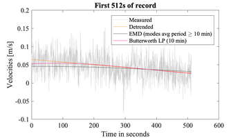
Zoom of the first 512 s segment of the measured velocities shown above including the same trends -
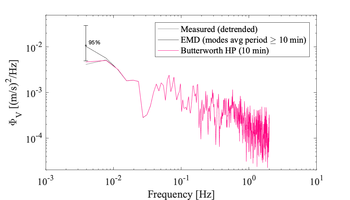
Example velocity spectra of the short 512 s of records before and after different detrending techniques applied to the original 6h time series. The impact of the detrending method can be seen at the lowest frequencies only


Trade-offs when choosing segment length
The shorter the segment, the higher the temporal resolution of the final time series.
Notes
- ↑ Zhaohua Wu, Norden E. Huang, Steven R. Long, and Chung-Kang Peng. 2007. On the trend, detrending, and variability of nonlinear and nonstationary time series. PNAS. doi:10.1073/pnas.0701020104

