Segmenting datasets

Once the raw observations have been quality-controlled, then you must split the time series into shorter segments by considering:

• Time and length scales of turbulence
• Stationarity of the segment and Taylor's frozen turbulence hypothesis
• Required statistical significance of the resulting spectra (important if you need to remove motion-induced contamination from the spectra)

Considerations

Measurements are typically collected in the following two ways:

• continuously, or in such long bursts that they can be considered continuous
• short bursts that are typically at most 2-3x the expected largest turbulence time scales (e.g., 10 min in ocean environments)

This segmenting step dictates the minimum burst duration when setting up your equipment. The act of chopping a time series into smaller subsets, i.e., segments, is effectively a form of low-pass (box-car) filtering. The length of the segment in time is usually a more important consideration than detrending the time series when estimating [math]\displaystyle{ \varepsilon }[/math] from the inertial subrange of the final spectra.

The shorter the segment, the higher the temporal resolution of the final [math]\displaystyle{ \varepsilon }[/math] time series, and the more likely the segment will be stationary. However, the spectrum's lowest resolved frequency and final resolution are the inverse of the fft-length, i.e., the duration of the signal used to construct the spectrum. Therefore, the segment must remain sufficiently long such that the lowest wavenumber (frequencies) of the inertial subrange are retained by the spectra. This is particularly important when measurement noise drowns the highest wavenumber (frequencies) of the inertial subrange. Thus, using too short segments may inadvertently render the spectra unusable for deriving [math]\displaystyle{ \varepsilon }[/math] from the inertial subrange by virtue of no longer resolving this subrange.

Contours represent the log of the fft-length required to resolve the non-dimensional wavenumber [rad/m] indicated in each panel's title. The inertial subrange ends at approximately [math]\displaystyle{ \hat{k}L_k\approx0.1 }[/math] (or [math]\displaystyle{ kL_k\approx0.015 }[/math] in cpm), and so panel (c) denotes the fft-length that resolves the end of the inertial subrange i.e., the beginning of the viscous subrange. The fft-length must be at least 10x longer (see b), preferably 50x (panel c) given the low number of spectral observations at the lowest frequencies (wavenumbers)

Recommendations

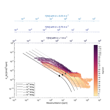
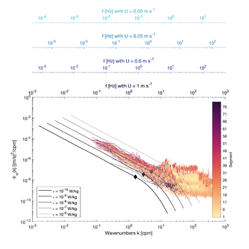
A good rule of thumb for tidally-influenced environments is 5 to 15 min segments, but this may be shorter in certain energetic and fast-moving flows (Fig. 1) and longer in less energetic environments (Fig.2). Are the peaks in the MAVS data vortex shedding from the rings. Check the motion sensors onboard?

Fig. 1: Example theoretical velocity spectra for different [math]\displaystyle{ \varepsilon }[/math] with the empirical limit [math]\displaystyle{ \hat{k}L_k\sim0.1 }[/math] denoted by the diamonds ([math]\displaystyle{ \hat{k} }[/math] is in rad/m). The inertial subrange extends to smaller wavenumber [math]\displaystyle{ k }[/math] [cpm] as [math]\displaystyle{ \varepsilon }[/math] increases. The lowest frequency resolved by a spectra is the inverse of the fft-length used when computing the spectra. The colored lines are spectral observations from a dataset with fast speeds and large [math]\displaystyle{ \varepsilon }[/math]. In this example, we used relatively short segments (128s) to estimate the spectra from fft-length of 32 s (2048 samples @ 64 Hz). The impact of turbulence anisotropy is also visible through the flattening of the spectra around 1 cpm. The secondary x-axis show the corresponding frequencies for a range of mean speeds past the sensors

Fig. 2: Same as Fig 1 but for a different dataset with low speeds and low [math]\displaystyle{ \varepsilon }[/math], requiring the use of relatively long segments (1024s) to estimate the spectra from fft-length of 512 s (4096 samples @ 8 Hz).

---

Return to Preparing_quality-controlled_velocities