Segmenting datasets

Once the raw observations have been quality-controlled, then you must split the time series into shorter segments by considering:

• Time and length scales of turbulence
• Stationarity of the segment and Taylor's frozen turbulence hypothesis
• Required statistical significance of the resulting spectra, important mainly if you use cospectral or coherence-based methods to remove motion-induced contamination from the spectra

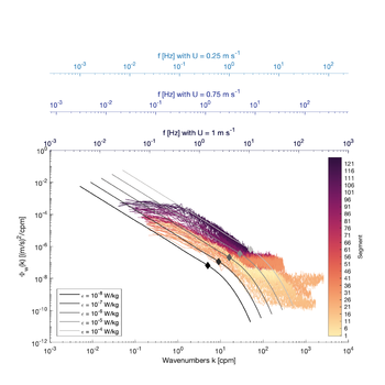
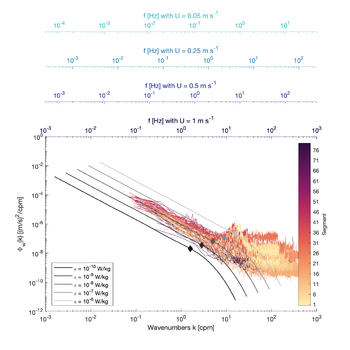
A good way to select the segment length is by inspecting the computed spectra estimated from a  512-s long segment and an fft-length that is one-quarter of the segment length (128 s). Plotting these spectra against the theoretical spectral lines (see Fig 2 and 3), enables identifying whether 1 decade of an inertial subrange is resolved with at least 8 spectral samples in this subrange. 

Considerations

Measurements are typically collected in the following two ways:

• continuously, or in such long bursts that they can be considered continuous
• short bursts that are typically at most 2-3x the expected largest turbulence time scales (e.g., 10 min in ocean environments)

This segmenting step dictates the minimum burst duration when setting up your equipment. The act of chopping a time series into smaller subsets, i.e., segments, is effectively a form of low-pass (box-car) filtering. The length of the segment in time is usually a more important consideration than detrending the time series when estimating [math]\displaystyle{ \varepsilon }[/math] from the inertial subrange of the final spectra.

The shorter the segment, the higher the temporal resolution of the final [math]\displaystyle{ \varepsilon }[/math] time series, and the more likely the segment will be stationary. The segment must remain sufficiently long such that the lowest wavenumber (frequencies) of the inertial subrange are retained by the computed spectra. This is particularly important when measurement noise drowns the highest wavenumber (frequencies) of the inertial subrange. Thus, using too short segments may inadvertently render the spectra unusable for deriving [math]\displaystyle{ \varepsilon }[/math] from the inertial subrange by virtue of no longer resolving this subrange as shown in (Fig. 1).

Fig.1 Contours represent the log of the fft-length required to resolve the non-dimensional wavenumber [rad/m] indicated in each panel's title. The inertial subrange ends at approximately [math]\displaystyle{ \hat{k}L_k\approx0.1 }[/math] (or [math]\displaystyle{ kL_k\approx0.015 }[/math] in cpm), and so panel (c) denotes the fft-length that resolves the end of the inertial subrange i.e., the beginning of the viscous subrange. The fft-length must be at least 10x longer (see b), preferably 50x (panel c) given the low number of spectral observations at the lowest frequencies (wavenumbers)

Recommendations

A good rule of thumb for tidally-influenced environments is 5 to 15 min segments, but this may be shorter in certain energetic and fast-moving flows (Fig. 2) and longer in less energetic environments (Fig.3). The final segment length is partly a function of the fft-length and the desired statistical significance (degrees of freedom) of the final computed spectra. If cospectral methods will be employed to decontaminate the velocities, then the segment length should be 4-5x larger than the fft-length unless band-averaging is used to average the (co-)spectra.

Minimum fft-length

Fig. 1 provides a guide to the fft-length required for resolving different subrange as a function of the speed past the sensor, and [math]\displaystyle{ \varepsilon }[/math]. For instance, an fft-length of 4 s would resolve one decade of the inertial subrange at speeds past the sensor of 0.5 m/s and [math]\displaystyle{ \varepsilon\sim10^{-7} }[/math] W/kg. Longer segments would be required for slower flows or lower [math]\displaystyle{ \varepsilon }[/math]. At [math]\displaystyle{ \varepsilon\approx10^{-9} }[/math] W/kg, one decade of the inertial subrange would be resolved with an fft-length longer than 10s provided the speed was faster than 0.5 m/s.

Because the inertial subrange may be contaminated at the highest wavenumbers by instrument noise, we suggest using longer segments than the minimum shown in Fig. 1b. This strategy also enables having a larger number of spectral observations to fit over the inertial subrange given the spectral resolution also depends on the fft-length.

Choosing segment-length

The final segment length may be larger than the fft-length depending if you use block-averaging for computing the spectra. The maximum segment length should be shorter than the largest turbulent time scales. To increase the statistical reliability of the spectral observations, which is absolutely necessary when applying any co-spectral techniques for motion decontamination of spectra, we recommend segment length that is 5x the fft-length unless band-averaging is employed during the spectral averaging. More details about the minimum degrees of freedom are given in the [[[velocity decontamination by cospectral methods]] wikipage.

Are the peaks in the MAVS data vortex shedding from the rings. Check the motion sensors onboard?

Fig. 2: Example theoretical velocity spectra for different [math]\displaystyle{ \varepsilon }[/math] with the empirical limit [math]\displaystyle{ \hat{k}L_k\sim0.1 }[/math] denoted by the diamonds ([math]\displaystyle{ \hat{k} }[/math] is in rad/m). The inertial subrange extends to smaller wavenumber [math]\displaystyle{ k }[/math] [cpm] as [math]\displaystyle{ \varepsilon }[/math] increases. The lowest frequency resolved by a spectra is the inverse of the fft-length used when computing the spectra. The colored lines are spectral observations from a dataset with fast speeds and large [math]\displaystyle{ \varepsilon }[/math]. In this example, we used relatively short segments (128s) to estimate the spectra from fft-length of 32 s (2048 samples @ 64 Hz). The impact of turbulence anisotropy is also visible through the flattening of the spectra around 1 cpm. The secondary x-axis show the corresponding frequencies for a range of mean speeds past the sensors

Fig. 3: Same as Fig 1 but for a different dataset with low speeds and low [math]\displaystyle{ \varepsilon }[/math], requiring the use of relatively long segments (1024s) to estimate the spectra from fft-length of 512 s (4096 samples @ 8 Hz).

Overlapping segments

Using overlapping segments, i.e., obtaining your first [math]\displaystyle{ \varepsilon }[/math] estimate from time 0 to 5 min, and the second estimate from 2.5 to 5 min (50% overlap) essentially smoothes the final timeseries [math]\displaystyle{ \varepsilon }[/math]. One advantage of using overlapping segments is that you can recover estimates before and after sudden changes in flow conditions that render one segment unusable for getting [math]\displaystyle{ \varepsilon }[/math]. The use of overlapping segments is purely a matter of preference, and does not impact the quality of the final timeseries of epsilon.

---

Return to Preparing quality-controlled velocities